rsyncrosim: introduction to ST-Sim
Source:vignettes/a05_rsyncrosim_stsim_vignette.Rmd
a05_rsyncrosim_stsim_vignette.RmdThis vignette will cover how to develop and run spatially-explicit,
stochastic state-and-transition simulation models of landscape change
using the rsyncrosim package within the
SyncroSim software
framework. For an overview of
SyncroSim and
rsyncrosim, as well as a basic usage tutorial for
rsyncrosim, see the
Introduction
to rsyncrosim vignette.
SyncroSim Package: stsim
To demonstrate how to create and run spatially-explicit, stochastic
state-and-transition simulation models (STSMs) of landscape change, we
will be using the
stsim
SyncroSim package. STSMs are well-suited for integrating uncertainty
into model projections, and have been applied to a variety of landscapes
and management questions. In this stsim example below, we
will model changes in forest cover types under two scenarios: no harvest
within a landscape, and harvest of 20 acres per year. To do this, we
will set a number of model parameters describing how many timesteps and
iterations the model will run for, transition types and their
probabilities, transition targets (particularly, for the harvest
transition type), etc. Next, we will provide stsim with a
set of initial conditions that describe the starting landscape at time
0, and specify parameters for the model’s output. After running both
scenarios, we will view the output data in tabular form and as a raster
layer. Spatial and non-spatial examples of this exercise are
provided.
For more details on stsim, consult the
ST-Sim online
documentation.
Setup
Install SyncroSim
Before using rsyncrosim you will first need to
download and
install the SyncroSim software. Versions of SyncroSim exist for both
Windows and Linux.
Note: this tutorial was developed using
rsyncrosim version 2.0. To use rsyncrosim
version 2.0 or greater, SyncroSim version 3.0 or greater is
required.
Installing and loading R packages
You will need to install the rsyncrosim R package,
either using
CRAN or from
the rsyncrosim
GitHub
repository. Versions of rsyncrosim are available for
both Windows and Linux. You may need to install the terra
package from CRAN as well.
In a new R script, load the necessary packages. This includes the
rsyncrosim and terra R packages.
# Load R packages
library(rsyncrosim)  # package for working with SyncroSim
library(terra)       # package for working with spatial data
Connecting R to SyncroSim using session()
Finish setting up the R environment for the rsyncrosim
workflow by creating a SyncroSim Session object. Use the
session() function to connect R to your installed copy of
the SyncroSim software.
mySession <- session("path/to/install_folder")      # Create a Session based SyncroSim install folder
mySession <- session()                              # Using default install folder (Windows only)
mySession                                           # Displays the Session object
## class : Session
## filepath [character]: C:\PROGRA~1\SYNCRO~1
## silent [logical] : TRUE
## printCmd [logical] : FALSE
## condaFilepath [NULL]:Use the version() function to ensure you are using the
latest version of SyncroSim.
version(mySession)## [1] "3.1.27"Installing SyncroSim packages using
installPackage()
Install stsim using the rsyncrosim function
installPackage(). This function takes a package name as
input and then queries the SyncroSim package server for the specified
package.
# Install stsim
installPackage("stsim")
## Package <stsim v4.5.3> installedstsim should now be included in the package list
returned by the packages() function in
rsyncrosim:
# Get list of installed packages
packages()
## name version description
## 1 stsim 4.5.3 The ST-Sim state-and-transition simulation model
## location
## 1 C:\\Users\\VickiZhang\\AppData\\Local\\SyncroSim\\Packages\\stsim\\4.5.3
## status
## 1 OKCreate a modeling workflow
When creating a new modeling workflow from scratch, we need to create objects of the following scopes:
For more information on these scopes, see the
Introduction
to rsyncrosim vignette.
Set up library, project, and scenario
# Create a new library
myLibrary <- ssimLibrary(name = "stsimLibrary.ssim",
                         session = mySession,
                         packages = "stsim")
## Package <stsim v4.5.3> addedView model inputs using datasheet()
View the datasheets associated with your new project and scenario
using the datasheet() function from
rsyncrosim.
# View all datasheets associated with a library, project, or scenario
datasheet_list <- datasheet(myScenario)
head(datasheet_list)
## scope name displayName
## 53 scenario core_DistributionValue Distributions
## 54 scenario core_ExternalVariableValue External Variables
## 55 scenario core_Pipeline Pipeline
## 56 scenario core_SpatialMultiprocessing Spatial Multiprocessing
## 57 scenario stsim_DeterministicTransition States
## 58 scenario stsim_DigitalElevationModel Digital Elevation Model
tail(datasheet_list)## scope name
## 144 scenario stsim_TransitionSpatialInitiationMultiplierFineRes
## 145 scenario stsim_TransitionSpatialMultiplier
## 146 scenario stsim_TransitionSpatialMultiplierFineRes
## 147 scenario stsim_TransitionSpreadDistribution
## 148 scenario stsim_TransitionTarget
## 149 scenario stsim_TransitionTargetPrioritization
## displayName
## 144 Transition Spatial Initiation Multipliers
## 145 Transition Spatial Multipliers
## 146 Transition Spatial Multipliers
## 147 Transition Spread Distribution
## 148 Transition Targets
## 149 Transition Target PrioritizationFrom this list of datasheets, we can check which datasheets specific
to the stsim package we would like to modify. This will
include a number of Initial Conditions datasheets, Output datasheets,
and a Run Control datasheet. For more information about all
stsim datasheets, see
the
online documentation.
Configure model inputs using datasheet() and
addRow()
Now, we will add some values to these datasheets so we can run our models.
Inputs for stsim come in two forms: scenario inputs
(which can vary by scenario) and project inputs (which
must be fixed across all scenarios). In general most inputs are
scenario inputs; project inputs are typically reserved for values that
must be shared by all scenarios (e.g. constants, shared lookup values).
We refer to project input datasheets as project-scoped
datasheets and scenario input datasheets as scenario-scoped
datasheets. We will start by retrieving some project-scoped input
datasheets to add and edit their values.
Project-scoped datasheets
Terminology: The project-scoped datasheet called
Terminology specifies terms used across all scenarios in
the same project.
# Load the Terminology datasheet to a new R data frame
terminology <- datasheet(myProject, name = "stsim_Terminology")

# Check the columns of the Terminology data frame
str(terminology)
## 'data.frame': 1 obs. of 9 variables:
## $ AmountLabel : chr "Area"
## $ AmountUnits : Factor w/ 5 levels "acres","hectares",..: 1
## $ StateLabelX : chr "Class"
## $ StateLabelY : chr "Subclass"
## $ PrimaryStratumLabel : chr "Primary Stratum"
## $ SecondaryStratumLabel: chr "Secondary Stratum"
## $ TertiaryStratumLabel : chr "Tertiary Stratum"
## $ TimestepUnits : chr "Timestep"
## $ StockUnits : chr "Tons"We can change the terminology of the StateLabelX and
AmountUnits columns in this datasheet, and then save those
changes back to the SyncroSim library file.
# Edit the values of the StateLabelX and AmountUnits columns
terminology$AmountUnits <- "hectares"
terminology$StateLabelX <- "Forest Type"

# Saves edits as a SyncroSim datasheet
saveDatasheet(ssimObject = myProject,
              data = terminology,
              name = "stsim_Terminology")
## Datasheet <stsim_Terminology> savedSimilarly, we can edit other project-scoped datasheets for ‘stsim’.
Stratum: Primary Strata in the model
# Load a copy of the Stratum datasheet.
# To load an empty copy of this datasheet, specify the argument empty = TRUE
stratum <- datasheet(myProject, "stsim_Stratum", empty = TRUE)

# Use the addRow() to add a value to the stratum  data frame
stratum <- addRow(stratum, "Entire Forest")

# Save edits as a SyncroSim datasheet
saveDatasheet(myProject, stratum, "stsim_Stratum", force = TRUE)
## Datasheet <stsim_Stratum> savedStateLabelX: First dimension of labels for State Classes
It is also possible to add values to a datasheet without loading it
into R. Below we create a vector of forestTypes and add
this to the stsim_StateLabelX datasheet as a data frame
using saveDatasheet().
# Create a vector containing the State Class labels
forestTypes <- c("Coniferous", "Deciduous", "Mixed")

# Add values as a data frame to a SyncroSim datasheet
saveDatasheet(myProject,
              data.frame(Name = forestTypes),
              "stsim_StateLabelX",
              force = TRUE)
## Datasheet <stsim_StateLabelX> savedStateLabelY: Second dimension of labels for State Classes
# Add values as a data frame directly to an stsim datasheet
saveDatasheet(myProject,
              data.frame(Name = c("All")),
              "stsim_StateLabelY",
              force = TRUE)
## Datasheet <stsim_StateLabelY> savedState Classes: Combine StateLabelX and
StateLabelY, and assign each class a unique name and Id
# Create a new R data frame containing the names of the State Classes
# and their corresponding data
stateClasses <- data.frame(Name = forestTypes)
stateClasses$StateLabelXId <- stateClasses$Name
stateClasses$StateLabelYId <- "All"
stateClasses$Id <- c(1, 2, 3)

# Save stateClasses R data frame to a SyncroSim datasheet
saveDatasheet(myProject, stateClasses, "stsim_StateClass", force = TRUE)
## Datasheet <stsim_StateClass> savedTransition Types: Assign a unique name and Id to each type of transition in our model.
# Create an R data frame containing transition type data
transitionTypes <- data.frame(Name = c("Fire", "Harvest", "Succession"),
                              Id = c(1, 2, 3))

# Save transitionTypes R data frame to a SyncroSim datasheet
saveDatasheet(myProject, transitionTypes, "stsim_TransitionType", force = TRUE)
## Datasheet <stsim_TransitionType> savedTransition Groups: Create Transition Groups identical to the Types
# Create an R data frame containing a column of transition type names
transitionGroups <- data.frame(Name = c("Fire", "Harvest", "Succession"))

# Save transitionGroups R data frame to a SyncroSim datasheet
saveDatasheet(myProject, transitionGroups, "stsim_TransitionGroup", force = T)
## Datasheet <stsim_TransitionGroup> savedTransition Types by Groups: Assign each Type to its Group
# Create an R data frame that contains Transition Type Group names
transitionTypesGroups <- data.frame(TransitionTypeId = transitionTypes$Name,
                                    TransitionGroupId = transitionGroups$Name)

# Save transitionTypesGroups R data frame to a SyncroSim datasheet
saveDatasheet(myProject,
              transitionTypesGroups,
              "stsim_TransitionTypeGroup",
              force = T)
## Datasheet <stsim_TransitionTypeGroup> savedAges: Define the basic parameters to control the age reporting in the model
# Define values for age reporting
ageFrequency <- 1
ageMax <- 101
ageGroups <- c(20, 40, 60, 80, 100)

# Add values as R data frames to the appropriate SyncroSim datasheet
saveDatasheet(myProject,
              data.frame(Frequency = ageFrequency, MaximumAge = ageMax),
              "stsim_AgeType",
              force = TRUE)
## Datasheet <stsim_AgeType> saved
saveDatasheet(myProject,
              data.frame(MaximumAge = ageGroups),
              "stsim_AgeGroup",
              force = TRUE)
## Datasheet <stsim_AgeGroup> savedScenario-scoped datasheets
Now that we have defined all our project-scoped input datasheets, we
can move on to specifying scenario-specific model inputs. We begin by
using the scenario function to create a new scenario in our
project.
# Create a new SyncroSim scenario
myScenario <- scenario(myProject, "No Harvest")
Once again we can use the datasheet() function (with
summary=TRUE) to display all the scenario-scoped
datasheets.
# Subset the full datasheet list to show only scenario-scoped datasheets
scenario_datasheet_list <- subset(datasheet(myScenario, summary = TRUE),
                                  scope == "scenario")

head(scenario_datasheet_list)
## scope name displayName
## 53 scenario core_DistributionValue Distributions
## 54 scenario core_ExternalVariableValue External Variables
## 55 scenario core_Pipeline Pipeline
## 56 scenario core_SpatialMultiprocessing Spatial Multiprocessing
## 57 scenario stsim_DeterministicTransition States
## 58 scenario stsim_DigitalElevationModel Digital Elevation Model
tail(scenario_datasheet_list)## scope name
## 144 scenario stsim_TransitionSpatialInitiationMultiplierFineRes
## 145 scenario stsim_TransitionSpatialMultiplier
## 146 scenario stsim_TransitionSpatialMultiplierFineRes
## 147 scenario stsim_TransitionSpreadDistribution
## 148 scenario stsim_TransitionTarget
## 149 scenario stsim_TransitionTargetPrioritization
## displayName
## 144 Transition Spatial Initiation Multipliers
## 145 Transition Spatial Multipliers
## 146 Transition Spatial Multipliers
## 147 Transition Spread Distribution
## 148 Transition Targets
## 149 Transition Target PrioritizationWe can now use the datasheet() function to retrieve, one
at a time, each of our scenario-scoped datasheets from our library.
Run Control: Define the length of the run and whether or not it is a spatial run (requires spatial inputs to be set, see below). Here we make the run spatial.
# Create an R data frame specifying to run the simulation for
# 7 realizations and 10 timesteps
runControl <- data.frame(MaximumIteration = 7,
                         MinimumTimestep = 0,
                         MaximumTimestep = 10,
                         IsSpatial = TRUE)

# Save transitionTypesGroups R data frame to a SyncroSim datasheet
saveDatasheet(myScenario, runControl, "stsim_RunControl",append = FALSE)
## Datasheet <stsim_RunControl> savedDeterministic Transitions: Define transitions that take place in the absence of probabilistic transitions. Here we also set the age boundaries for each State Class.
# Load  an empty Deterministic Transitions datasheet to a new R data frame
dTransitions <- datasheet(myScenario,
                          "stsim_DeterministicTransition",
                          optional = T,
                          empty = T,
                          lookupsAsFactors = F)

# Add all Deterministic Transitions to the R data frame
dTransitions <- addRow(dTransitions, data.frame(
  StateClassIdSource = "Coniferous",
  StateClassIdDest = "Coniferous",
  AgeMin = 21,
  Location = "C1"))
dTransitions <- addRow(dTransitions, data.frame(
  StateClassIdSource = "Deciduous",
  StateClassIdDest = "Deciduous",
  Location = "A1"))
dTransitions <- addRow(dTransitions, data.frame(
  StateClassIdSource = "Mixed",
  StateClassIdDest = "Mixed",
  AgeMin = 11,
  Location = "B1"))

# Save dTransitions R data frame to a SyncroSim datasheet
saveDatasheet(myScenario, dTransitions, "stsim_DeterministicTransition")
## Datasheet <stsim_DeterministicTransition> savedProbabilistic Transitions: Define transitions between State Classes and assigns a probability to each.
# Load  an empty Probabilistic Transitions datasheet to a new R data frame
pTransitions <- datasheet(myScenario,
                          "stsim_Transition",
                          optional = T,
                          empty = T,
                          lookupsAsFactors = F)

# Add all Probabilistic Transitions to the R data frame
pTransitions <- addRow(pTransitions, data.frame(
  StateClassIdSource = "Coniferous",
  StateClassIdDest = "Deciduous",
  TransitionTypeId = "Fire",
  Probability = 0.01))
pTransitions <- addRow(pTransitions, data.frame(
  StateClassIdSource = "Coniferous",
  StateClassIdDest = "Deciduous",
  TransitionTypeId = "Harvest",
  Probability = 1,
  AgeMin = 40))
pTransitions <- addRow(pTransitions, data.frame(
  StateClassIdSource = "Deciduous",
  StateClassIdDest = "Deciduous",
  TransitionTypeId = "Fire",
  Probability = 0.002))
pTransitions <- addRow(pTransitions, data.frame(
  StateClassIdSource = "Deciduous",
  StateClassIdDest = "Mixed",
  TransitionTypeId = "Succession",
  Probability = 0.1,
  AgeMin = 10))
pTransitions <- addRow(pTransitions, data.frame(
  StateClassIdSource = "Mixed",
  StateClassIdDest = "Deciduous",
  TransitionTypeId = "Fire",
  Probability = 0.005))
pTransitions <- addRow(pTransitions, data.frame(
  StateClassIdSource = "Mixed",
  StateClassIdDest = "Coniferous",
  TransitionTypeId = "Succession",
  Probability = 0.1,
  AgeMin = 20))

# Save pTransitions R data frame to a SyncroSim datasheet
saveDatasheet(myScenario, pTransitions, "stsim_Transition")
## Datasheet <stsim_Transition> savedInitial Conditions: Set the starting conditions of the model at time 0. There are two options for setting initial conditions: either spatial or non-spatial. In this example we will use spatial initial conditions; however, we also demonstrate how to set initial conditions non-spatially below.
-
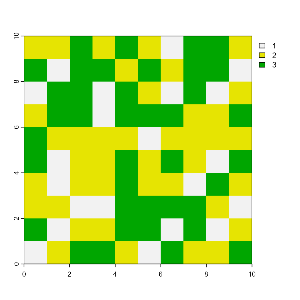
Option 1 - Spatial. Let’s first take a
look at our rasters. We will retrieve the sample raster files (in
GeoTIFF format) provided with the
rsyncrosimpackage.
# Load sample .tif files
stratumTif <- "initial-stratum.tif"
sclassTif <- "initial-sclass.tif"
ageTif <- "initial-age.tif"
# Create raster layers from the .tif files
rStratum <- rast(stratumTif)
rSclass <- rast(sclassTif)
rAge <- rast(ageTif)

# Plot raster layers
plot(rStratum)
plot(rSclass)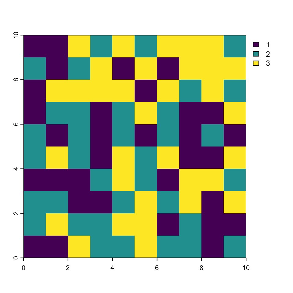
plot(rAge)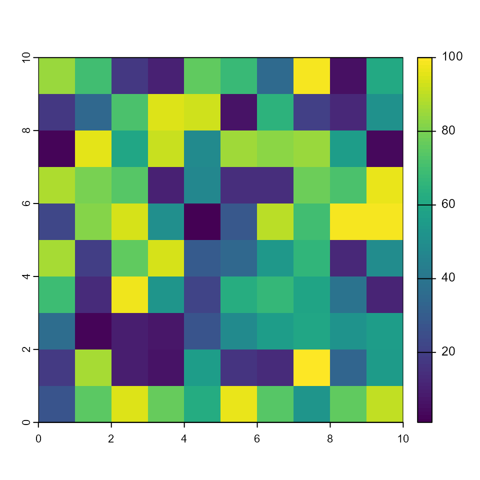
We can add these rasters as model inputs using the
stsim_InitialConditionsSpatial datasheet.
# Create an data.frame of the input raster layers
ICSpatial <- data.frame(StratumFileName = stratumTif,
                  StateClassFileName = sclassTif,
                  AgeFileName = ageTif)

# Save initialConditionsSpatial R list to a SyncroSim datasheet
saveDatasheet(myScenario, ICSpatial, "stsim_InitialConditionsSpatial")
## Datasheet <stsim_InitialConditionsSpatial> saved-
Option 2 - Non-spatial. The second option
is to set the proportions of each class, making this a non-spatial
parameterization. To do so, we use the
stsim_InitialConditionsNonSpatialandstsim_InitialConditionsNonSpatialDistributiondatasheets:
# Create non-spatial initial conditions data and add it to an R data frame
ICNonSpatial <- data.frame(TotalAmount = 100,
                           NumCells = 100,
                           CalcFromDist = F)

# Save the ICNonSpatial R data frame to a SyncroSim datasheet
saveDatasheet(myScenario, ICNonSpatial, "stsim_InitialConditionsNonSpatial")
## Datasheet <stsim_InitialConditionsNonSpatial> saved
# Create non-spatial initial conditions distribution data and add it to an R data frame
ICNonSpatialDistribution <- data.frame(StratumId = "Entire Forest",
                                       StateClassId = "Coniferous",
                                       RelativeAmount = 1)

# Save the ICNonSpatial R data frame to a SyncroSim datasheet
saveDatasheet(myScenario, ICNonSpatialDistribution,
              "stsim_InitialConditionsNonSpatialDistribution")
## Datasheet <stsim_InitialConditionsNonSpatialDistribution> savedTransition Targets: Define targets, in units of area, to be reached by the allocation procedure within SyncroSim.
# Set the transition target for harvest to 0
saveDatasheet(myScenario,
              data.frame(TransitionGroupId = "Harvest",
                         Amount = 0),
              "stsim_TransitionTarget")
## Datasheet <stsim_TransitionTarget> savedOutput Options: Regulate the model outputs and determine the frequency at which syncrosim saves the model outputs.
# Create output options for spatial model and add it to an R data frame
outputOptionsSpatial <- data.frame(
  RasterOutputSC = T, RasterOutputSCTimesteps = 1,
  RasterOutputTR = T, RasterOutputTRTimesteps = 1,
  RasterOutputAge = T, RasterOutputAgeTimesteps = 1
)

# Save the outputOptionsSpatial R data frame to a SyncroSim datasheet
saveDatasheet(myScenario, outputOptionsSpatial, "stsim_OutputOptionsSpatial")
## Datasheet <stsim_OutputOptionsSpatial> saved
# Create output options for non-spatial model and add it to an R data frame
outputOptionsNonSpatial <- data.frame(
  SummaryOutputSC = T, SummaryOutputSCTimesteps = 1,
  SummaryOutputTR = T, SummaryOutputTRTimesteps = 1
)

# Save the outputOptionsNonSpatial R data frame to a SyncroSim datasheet
saveDatasheet(myScenario, outputOptionsNonSpatial, "stsim_OutputOptions")
## Datasheet <stsim_OutputOptions> savedPipeline datasheet: Specify which transformer stage the scenarios will run and in which order.
To learn more about pipelines, see the rsyncrosim:
introduction to pipelines vignette and the SyncroSim
Enhancing
a Package: Linking Models tutorial.
To implement pipelines in our package, we need to specify the order
in which to run the transformers (i.e. models) in our pipeline by
editing the Pipeline datasheet. The Pipeline
datasheet is part of the built-in SyncroSim core, so we access it using
the “core_” prefix with the datasheet() function.
From viewing the structure of the Pipeline datasheet we
know that the StageNameId is a factor with a single level:
ST-Sim.
# Load Pipeline datasheet to an R data frame
myPipelineDataframe <- datasheet(myScenario, name = "core_Pipeline")

# Check the columns of the Pipeline data frame
str(myPipelineDataframe)
## 'data.frame': 0 obs. of 2 variables:
## $ StageNameId: Factor w/ 1 level "ST-Sim":
## $ RunOrder : num
# Create Pipeline data and add it to the Pipeline data frame
myPipelineRow <- data.frame(StageNameId = c("ST-Sim"),
                            RunOrder = c(1))

myPipelineDataframe <- addRow(myPipelineDataframe, myPipelineRow)

# Check values
myPipelineDataframe
## StageNameId RunOrder
## 1 ST-Sim 1
# Save Pipeline R data frame to a SyncroSim datasheet
saveDatasheet(ssimObject = myScenario,
              data = myPipelineDataframe,
              name = "core_Pipeline")
## Datasheet <core_Pipeline> savedWe are done parameterizing our simple “No Harvest” scenario. Let’s now define a new scenario that implements forest harvesting. Below, we create a second “Harvest” scenario that is a copy of the first scenario, but with a harvest level of 20 acres/year.
# Create a copy of the no harvest scenario (i.e myScenario) and name it myScenarioHarvest
myScenarioHarvest <- scenario(myProject,
                              scenario = "Harvest",
                              sourceScenario = myScenario)

# Set the transition target for harvest to 20 acres/year
saveDatasheet(myScenarioHarvest,
              data.frame(TransitionGroupId = "Harvest", Amount = 20),
              "stsim_TransitionTarget")
## Datasheet <stsim_TransitionTarget> savedWe can display the harvest levels for both scenarios.
# View the transition targets for the Harvest and No Harvest scenarios
datasheet(myProject,
          scenario = c("Harvest", "No Harvest"),
          name = "stsim_TransitionTarget")
## ScenarioId ProjectId ScenarioName ParentId ParentName TransitionGroupId
## 1 2 1 No Harvest NA <NA> Harvest
## 2 3 1 Harvest NA <NA> Harvest
## 3 2 1 No Harvest NA <NA> Harvest
## 4 3 1 Harvest NA <NA> Harvest
## Amount
## 1 0
## 2 0
## 3 20
## 4 20Run Scenarios
Setting the number of multiprocessing jobs
If we have a large model and we want to parallelize the run using multiprocessing, we can modify the library-scoped “core_Multiprocessing” datasheet. Since we are using five iterations in our model, we will set the number of jobs to five so each multiprocessing core will run a single iteration.
# Load list of available library-scoped datasheets
datasheet(myLibrary)
## scope name displayName
## 1 library core_Backup Backup
## 2 library core_JlConfig Julia
## 3 library core_Multiprocessing Multiprocessing
## 4 library core_Option Options
## 5 library core_ProcessorGroupOption Processor Group Options
## 6 library core_ProcessorGroupValue Processor Group Values
## 7 library core_PublishDatasheet PublishDatasheet
## 8 library core_PyConfig Python
## 9 library core_RConfig R
## 10 library core_Setting Settings
## 11 library core_SpatialMultiprocessingOption Spatial Multiprocessing Option
## 12 library core_SpatialOption Spatial Options
## 13 library core_SysFolder Folders
## 14 library core_Terminology Terminology
# Load the library-scoped multiprocessing datasheet
multiprocess <- datasheet(myLibrary, name = "core_Multiprocessing")
## [1] "Note: MaximumJobs should be between 1 and 9999"
# Check required inputs
str(multiprocess)
## 'data.frame': 1 obs. of 4 variables:
## $ EnableMultiprocessing : logi FALSE
## $ MaximumJobs : num 15
## $ EnableMultiScenario : logi FALSE
## $ EnableCopyExternalFiles: logi NA
# Enable multiprocessing
multiprocess$EnableMultiprocessing <- TRUE

# Set maximum number of jobs to 5
multiprocess$MaximumJobs <- 4

# Save multiprocessing configuration
saveDatasheet(ssimObject = myLibrary,
              data = multiprocess,
              name = "core_Multiprocessing")
## Datasheet <core_Multiprocessing> savedSetting run parameters with run()
Now, when we run our scenario, it will use the desired multiprocessing configuration. Running a scenario generates a corresponding new child scenario, called a results scenario, which contains the results of the run along with a snapshot of all the model inputs.
# Run both scenarios
myResultScenario <- run(myProject,
                        scenario = c("Harvest", "No Harvest"),
                        summary = TRUE)
## [1] "Running scenario [3] Harvest"
## [1] "Running scenario [2] No Harvest"View results
The next step is to view the output datasheets added to the result
scenario when it was run. To look at the results we first need to
retrieve the unique scenarioId for each child result
scenario.
# Retrieve scenario IDs
resultIDNoHarvest <- subset(myResultScenario,
                            ParentId == scenarioId(myScenario))$ScenarioId
resultIDHarvest <- subset(myResultScenario,
                          ParentId == scenarioId(myScenarioHarvest))$ScenarioId
We can now retrieve tabular output regarding the projected State
Class over time (for both scenarios combined) from the
stsim_OutputStratumState datasheet.
# Retrieve output projected State Class for both Scenarios in tabular form
outputStratumState <- datasheet(
  myProject,
  scenario = c(resultIDNoHarvest, resultIDHarvest),
  name = "stsim_OutputStratumState")
Finally, we can get the State Class raster output using the
datasheetRaster() function (here for the Harvest scenario
only).
# Retrieve the output State Class raster for the Harvest scenario at timestep 5
myRastersTimestep5 <- datasheetSpatRaster(ssimObject = myProject,
                                          scenario = resultIDHarvest,
                                          datasheet = "stsim_OutputSpatialState",
                                          timestep = 5)
myRastersTimestep5
## class : SpatRaster
## size : 10, 10, 7 (nrow, ncol, nlyr)
## resolution : 1, 1 (x, y)
## extent : 0, 10, 0, 10 (xmin, xmax, ymin, ymax)
## coord. ref. : UTM Zone 10, Northern Hemisphere
## sources : sc.it1.ts5.tif
## sc.it2.ts5.tif
## sc.it3.ts5.tif
## ... and 4 more sources
## names : sc.it1.ts5, sc.it2.ts5, sc.it3.ts5, sc.it4.ts5, sc.it5.ts5, sc.it6.ts5, ...
# Plot raster for the first realization of timestep 5
plot(myRastersTimestep5[[1]])