rsyncrosim: introduction to spatial data
Source:vignettes/a04_rsyncrosim_vignette_spatial.Rmd
a04_rsyncrosim_vignette_spatial.RmdThis vignette will cover incorporating spatial data into SyncroSim
models using the rsyncrosim package within the
SyncroSim software
framework. For an overview of
SyncroSim and
rsyncrosim,
as well as a basic usage tutorial for rsyncrosim, see the
Introduction
to rsyncrosim vignette. To learn how to use iterations
in the rsyncrosim interface, see the
rsyncrosim:
introduction to uncertainty vignette. To learn how to link models
using pipelines in the rsyncrosim interface, see the
rsyncrosim:
introduction to pipelines vignette.
SyncroSim Package: helloworldSpatial
To demonstrate how to use spatial data in the rsyncrosim
interface, we will be using the
helloworldSpatial
SyncroSim package. helloworldSpatial was designed to be a
simple package to show off some key functionalities of SyncroSim,
including the ability to use both spatial and non-spatial data.
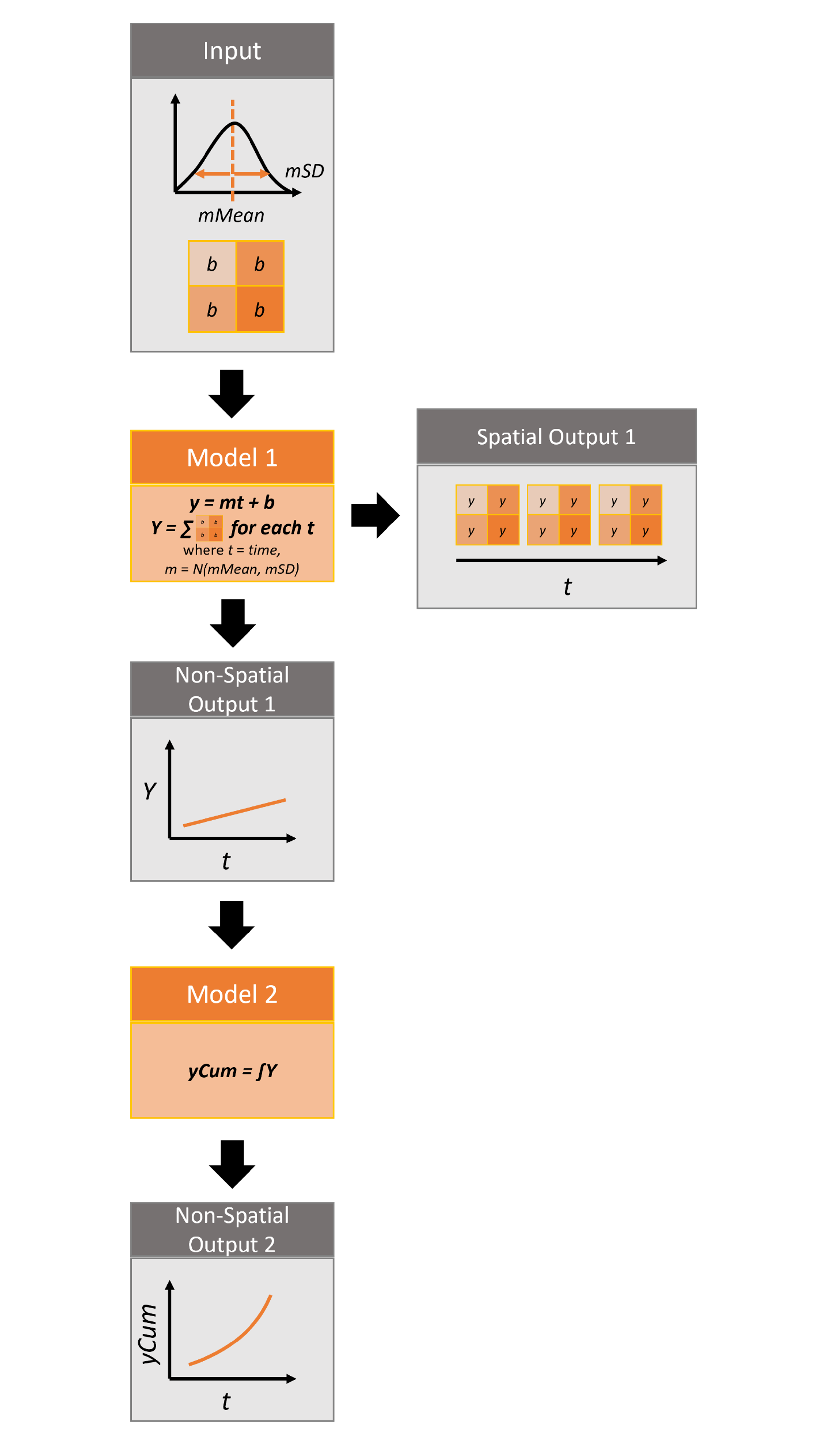
The package takes 3 inputs, mMean, mSD, and a spatial raster file of intercept (b) values. For each iteration, a value m, representing the slope, is sampled from a normal distribution with mean of mMean and standard deviation of mSD. These values are run through 2 models to produce both spatial and non-spatial outputs.
For more details on the different features of the
helloworldSpatial SyncroSim package, consult the SyncroSim
Enhancing
a Package: Integrating Spatial Data tutorial.
Setup
Install SyncroSim
Before using rsyncrosim you will first need to
download and
install the SyncroSim software. Versions of SyncroSim exist for both
Windows and Linux.
Note: this tutorial was developed using
rsyncrosim version 2.0. To use rsyncrosim
version 2.0 or greater, SyncroSim version 3.0 or greater is
required.
Installing and loading R packages
You will need to install the rsyncrosim R package,
either using
CRAN or from
the rsyncrosim
GitHub
repository. Versions of rsyncrosim are available for
both Windows and Linux. You may need to install the terra
package from CRAN as well.
In a new R script, load the necessary packages. This includes the
rsyncrosim and terra R packages.
# Load R packages
library(rsyncrosim)  # package for working with SyncroSim
library(terra)       # package for working with spatial data
Connecting R to SyncroSim using session()
Finish setting up the R environment for the rsyncrosim
workflow by creating a SyncroSim Session object. Use the
session() function to connect R to your installed copy of
the SyncroSim software.
mySession <- session("path/to/install_folder")      # Create a Session based SyncroSim install folder
mySession <- session()                              # Using default install folder (Windows only)
mySession                                           # Displays the Session object
## class : Session
## filepath [character]: C:\PROGRA~1\SYNCRO~1
## silent [logical] : TRUE
## printCmd [logical] : FALSE
## condaFilepath [NULL]:Use the version() function to ensure you are using the
latest version of SyncroSim.
version(mySession)## [1] "3.1.27"Installing SyncroSim packages using
installPackage()
Install helloworldSpatial using the
rynscrosim function installPackage(). This
function takes a package name as input and then queries the SyncroSim
package server for the specified package.
# Install helloworldSpatial
installPackage("helloworldSpatial")
## Package <helloworldSpatial v2.1.0> installedhelloworldSpatial should now be included in the package
list returned by the packages() function in
rsyncrosim:
# Get list of installed packages
packages()
## name version
## 1 helloworldSpatial 2.1.0
## description
## 1 Example demonstrating how to use spatial data with an R model
## location
## 1 C:\\Users\\VickiZhang\\AppData\\Local\\SyncroSim\\Packages\\helloworldSpatial\\2.1.0
## status
## 1 OKCreate a modeling workflow
When creating a new modeling workflow from scratch, we need to create objects of the following scopes:
For more information on these scopes, see the Introduction
to rsyncrosim vignette.
Set up library, project, and scenario
# Create a new library
myLibrary <- ssimLibrary(name = "helloworldLibrary.ssim",
                         session = mySession,
                         packages = "helloworldSpatial",
                         overwrite = TRUE)
## Package <helloworldSpatial v2.1.0> addedView model inputs using datasheet()
View the datasheets associated with your new scenario using the
datasheet() function from rsyncrosim.
# View all datasheets associated with a library, project, or scenario
datasheet(myScenario)
## scope name displayName
## 26 scenario core_DistributionValue Distributions
## 27 scenario core_ExternalVariableValue External Variables
## 28 scenario core_Pipeline Pipeline
## 29 scenario core_SpatialMultiprocessing Spatial Multiprocessing
## 30 scenario helloworldSpatial_InputDatasheet Inputs
## 31 scenario helloworldSpatial_IntermediateDatasheet Intermediate Outputs
## 32 scenario helloworldSpatial_OutputDatasheet Outputs
## 33 scenario helloworldSpatial_RunControl Run ControlFrom the list of datasheets above, we can see that there are four
datasheets specific to the helloworldSpatial package,
including an Inputs datasheet, an
Intermediate Outputs datasheet, an Outputs
datasheet, and a Run Control datasheet.
Configure model inputs using datasheet() and
addRow()
Currently our input scenario datasheets are empty! We need to add
some values to our Inputs datasheet,
Run Control datasheet, and Pipeline datasheet
so we can run our model.
Inputs datasheet
First, assign the contents of the Inputs datasheet to a
new data frame variable using datasheet(), then check the
columns that need input values.
# Load Inputs datasheet to a new R data frame
myInputDataframe <- datasheet(myScenario,
                              name = "helloworldSpatial_InputDatasheet")

# Check the columns of the input data frame
str(myInputDataframe)
## 'data.frame': 0 obs. of 3 variables:
## $ mMean : num
## $ mSD : num
## $ InterceptRasterFile: chrThe Inputs datasheet requires three values:
-
mMean: the mean of a normal distribution that will determine the slope of the linear equation. -
mSD: the standard deviation of a normal distribution that will determine the slope of the linear equation. -
InterceptRasterFile: the file path to a raster image, in which each cell of the image will be an intercept in the linear equation.
In this example, the external file we are using for the
InterceptRasterFile is a simple 5x5 raster TIF file
generated using the raster package in R. The file used in
this vignette can be found
here.
Add these values to a new data frame, then use the
addRow() function from rsyncrosim to update
the input data frame
# Create input data and add it to the input data frame
myInputRow <- data.frame(mMean = 0,
                         mSD = 4,
                         InterceptRasterFile = "path/to/input-raster.tif")
myInputDataframe <- addRow(myInputDataframe, myInputRow)

# Check values
myInputDataframe
## mMean mSD InterceptRasterFile
## 1 0 4 path/to/input-raster.tifFinally, save the updated R data frame to a SyncroSim datasheet using
saveDatasheet().
# Save input R data frame as a SyncroSim datasheet
saveDatasheet(ssimObject = myScenario,
              data = myInputDataframe,
              name = "helloworldSpatial_InputDatasheet")
## Datasheet <helloworldSpatial_InputDatasheet> savedRun Control datasheet
The Run Control datasheet sets the number of iterations
and the minimum and maximum time steps for our model. We’ll assign the
contents of this datasheet to a new data frame variable as well and then
add then update the information in the data frame using
addRow(). We need to specify data for the following four
columns:
-
MaximumIteration: total number of iterations to run the model for. -
MinimumTimestep: the starting time point of the simulation. -
MaximumTimestep: the end time point of the simulation.
Note: A fourth hidden column, MinimumIteration,
also exists in the Run Control datasheet (default=1).
# Load Run Control datasheet to an R data frame
runSettings <- datasheet(myScenario, name = "helloworldSpatial_RunControl")

# Check the columns of the Run Control data frame
str(runSettings)
## 'data.frame': 0 obs. of 3 variables:
## $ MinimumTimestep : num
## $ MaximumTimestep : num
## $ MaximumIteration: num
# Create Run Control data and add it to the Run Control data frame
runSettingsRow <- data.frame(MaximumIteration = 5,
                             MinimumTimestep = 1,
                             MaximumTimestep = 10)

runSettings <- addRow(runSettings, runSettingsRow)

# Check values
runSettings
## MinimumTimestep MaximumTimestep MaximumIteration
## 1 1 10 5
# Save Run Control R data frame to a SyncroSim datasheet
saveDatasheet(ssimObject = myScenario,
              data = runSettings,
              name = "helloworldSpatial_RunControl")
## Datasheet <helloworldSpatial_RunControl> savedPipeline datasheet
The helloworldSpatial package uses pipelines to link the
output of one model to the input of a second model. To learn more about
pipelines, see the rsyncrosim:
introduction to pipelines vignette and the SyncroSim
Enhancing
a Package: Linking Models tutorial.
To implement pipelines in our package, we need to specify the order
in which to run the transformers (i.e. models) in our pipeline by
editing the Pipeline datasheet. The Pipeline
datasheet is part of the built-in SyncroSim core, so we access it using
the “core_” prefix with the datasheet() function.
From viewing the structure of the Pipeline datasheet we
know that the StageNameId is a factor with two levels:
- Hello World Spatial 1 (R)
- Hello World Spatial 2 (R)
We will set the data for this datasheet such that
Hello World Spatial 1 (R) is run first, then
Hello World Spatial 2 (R). This way, the output from
Hello World Spatial 1 (R) is used as the input for
Hello World Spatial 2 (R).
# Load Pipeline datasheet to an R data frame
myPipelineDataframe <- datasheet(myScenario, name = "core_Pipeline")

# Check the columns of the Pipeline data frame
str(myPipelineDataframe)
## 'data.frame': 0 obs. of 2 variables:
## $ StageNameId: Factor w/ 2 levels "Hello World Spatial 1 (R)",..:
## $ RunOrder : num
# Create Pipeline data and add it to the Pipeline data frame
myPipelineRow <- data.frame(StageNameId = c("Hello World Spatial 1 (R)",
                                            "Hello World Spatial 2 (R)"),
                            RunOrder = c(1, 2))

myPipelineDataframe <- addRow(myPipelineDataframe, myPipelineRow)

# Check values
myPipelineDataframe
## StageNameId RunOrder
## 1 Hello World Spatial 1 (R) 1
## 2 Hello World Spatial 2 (R) 2
# Save Pipeline R data frame to a SyncroSim datasheet
saveDatasheet(ssimObject = myScenario, data = myPipelineDataframe,
              name = "core_Pipeline")
## Datasheet <core_Pipeline> savedRun scenarios
Setting the number of multiprocessing jobs
If we have a large model and we want to parallelize the run using multiprocessing, we can modify the library-scoped “core_Multiprocessing” datasheet. Since we are using five iterations in our model, we will set the number of jobs to five so each multiprocessing core will run a single iteration.
# Load list of available library-scoped datasheets
datasheet(myLibrary)
## scope name displayName
## 1 library core_Backup Backup
## 2 library core_JlConfig Julia
## 3 library core_Multiprocessing Multiprocessing
## 4 library core_Option Options
## 5 library core_ProcessorGroupOption Processor Group Options
## 6 library core_ProcessorGroupValue Processor Group Values
## 7 library core_PublishDatasheet PublishDatasheet
## 8 library core_PyConfig Python
## 9 library core_RConfig R
## 10 library core_Setting Settings
## 11 library core_SpatialMultiprocessingOption Spatial Multiprocessing Option
## 12 library core_SpatialOption Spatial Options
## 13 library core_SysFolder Folders
## 14 library core_Terminology Terminology
# Load the library-scoped multiprocessing datasheet
multiprocess <- datasheet(myLibrary, name = "core_Multiprocessing")
## [1] "Note: MaximumJobs should be between 1 and 9999"
# Check required inputs
str(multiprocess)
## 'data.frame': 1 obs. of 4 variables:
## $ EnableMultiprocessing : logi FALSE
## $ MaximumJobs : num 15
## $ EnableMultiScenario : logi FALSE
## $ EnableCopyExternalFiles: logi NA
# Enable multiprocessing
multiprocess$EnableMultiprocessing <- TRUE

# Set maximum number of jobs to 5
multiprocess$MaximumJobs <- 4

# Save multiprocessing configuration
saveDatasheet(ssimObject = myLibrary,
              data = multiprocess,
              name = "core_Multiprocessing")
## Datasheet <core_Multiprocessing> savedSetting run parameters with run()
Now, when we run our scenario, it will use the desired multiprocessing configuration.
# Run the first scenario we created
myResultScenario <- run(myScenario)
## [1] "Running scenario [1] My spatial scenario"## This model uses Conda environments, but no Conda installation was found. Using local environment.After the scenario has been run, a results scenario is created that contains results in the output datasheets.
View results
The next step is to view the output datasheets added to the result scenario when it was run.
Viewing non-spatial results with datasheet()
First, we will view the non-spatial results within the results
scenarios. For each step in the pipeline, We can load the result tables
using the datasheet() function.
# Load results of first transformer in the pipeline
resultsSummary <- datasheet(myResultScenario,
                            name = "helloworldSpatial_IntermediateDatasheet")

# View results table of first transformer in the pipeline
head(resultsSummary)
## Iteration Timestep y OutputRasterFile
## 1 1 1 104.0214 rasterMap_iter1_ts1.tif
## 2 1 2 212.3768 rasterMap_iter1_ts2.tif
## 3 1 3 320.7322 rasterMap_iter1_ts3.tif
## 4 1 4 429.0876 rasterMap_iter1_ts4.tif
## 5 1 5 537.4429 rasterMap_iter1_ts5.tif
## 6 1 6 645.7983 rasterMap_iter1_ts6.tif
# Load results of second transformer in the pipeline
resultsSummary2 <- datasheet(myResultScenario,
                             name = "helloworldSpatial_OutputDatasheet")

# View results table of second transformer in the pipeline
head(resultsSummary2)
## Iteration Timestep yCum
## 1 1 1 104.0214
## 2 1 2 316.3982
## 3 1 3 637.1303
## 4 1 4 1066.2179
## 5 1 5 1603.6608
## 6 1 6 2249.4592From viewing these datasheets, we can see that the spatial output is
contained within the IntermediateDatasheet, in the column
called OutputRasterFile.
Viewing spatial results with datasheetSpatRaster()
For spatial results, we want to load the results as raster images. To
do this, we will use the datasheetSpatRaster() function
from rsyncrosim. The first argument is the result
scenario object. Next, we specify the name of the datasheet
containing raster images using the datasheet argument, and
the column pertaining to the raster images using the column
argument. The results contain many raster images, since we have a raster
for each combination of iteration and timestep. We can use the
iteration and timestep arguments to specify a
single raster image or a subset of raster images we want to view.
# Load raster files for first result scenario with timestep and iteration
rasterMaps <- datasheetSpatRaster(
  myResultScenario,
  datasheet = "helloworldSpatial_IntermediateDatasheet",
  column = "OutputRasterFile",
  iteration = 1,
  timestep = 5
  )

# View results
rasterMaps
## class : SpatRaster
## size : 5, 5, 1 (nrow, ncol, nlyr)
## resolution : 0.4, 0.4 (x, y)
## extent : -1, 1, -1, 1 (xmin, xmax, ymin, ymax)
## coord. ref. : lon/lat WGS 84
## source : rasterMap_iter1_ts5.tif
## name : rasterMap_iter1_ts5
## min value : 19.04526
## max value : 23.78952
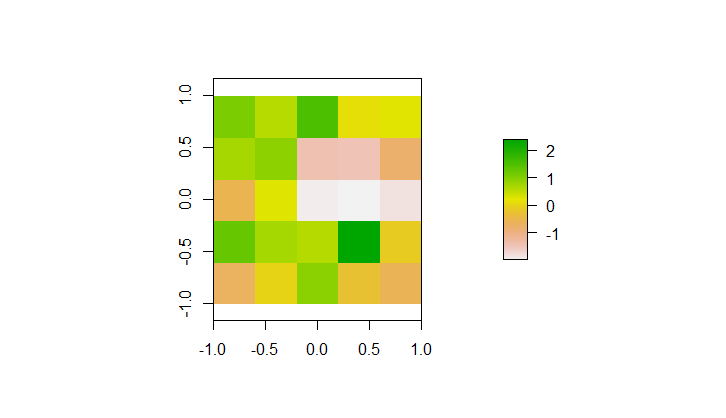
plot(rasterMaps[[1]])
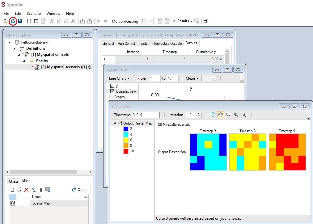
Viewing spatial results in SyncroSim Studio
To create maps using the results scenario we just generated, open the
current library in SyncroSim Studio and sync the updates from
rsyncrosim using the “refresh” button in the upper toolbar
(circled in red below). All the updates made in rsyncrosim
should appear in SyncroSim Studio. We can now add the results scenario
to the Results Viewer and create our maps. For more information on
generating map in SyncroSim Studio, see the SyncroSim tutorials on
creating
and
customizing
maps
rsyncrosim with SyncroSim
Studio to map spatial data