rsyncrosim: introduction to uncertainty
Source: vignettes/rsyncrosim_vignette_uncertainty.Rmd
rsyncrosim_vignette_uncertainty.RmdThis vignette will cover Monte Carlo realizations for modeling uncertainty using the rsyncrosim package within the SyncroSim software framework. For an overview of SyncroSim and rsyncrosim, as well as a basic usage tutorial for rsyncrosim, see the Introduction to rsyncrosim vignette.
SyncroSim Package: helloworldUncertainty
To demonstrate how to quantify model uncertainty using the rsyncrosim interface, we will need the helloworldUncertainty SyncroSim package. helloworldUncertainty was designed to be a simple package for introducing iterations to SyncroSim modeling workflows. The use of iterations allows for repeated simulations, known as “Monte Carlo realizations”, in which each simulation independently samples from a distribution of values.
The package takes from the user 3 inputs, mMean, mSD, and b. For each iteration, a value m, representing the slope, is sampled from a normal distribution with mean of mMean and standard deviation of mSD. The b value represents the intercept. These input values are run through a linear model, y=mt+b, where t is time, and the y value is returned as output.
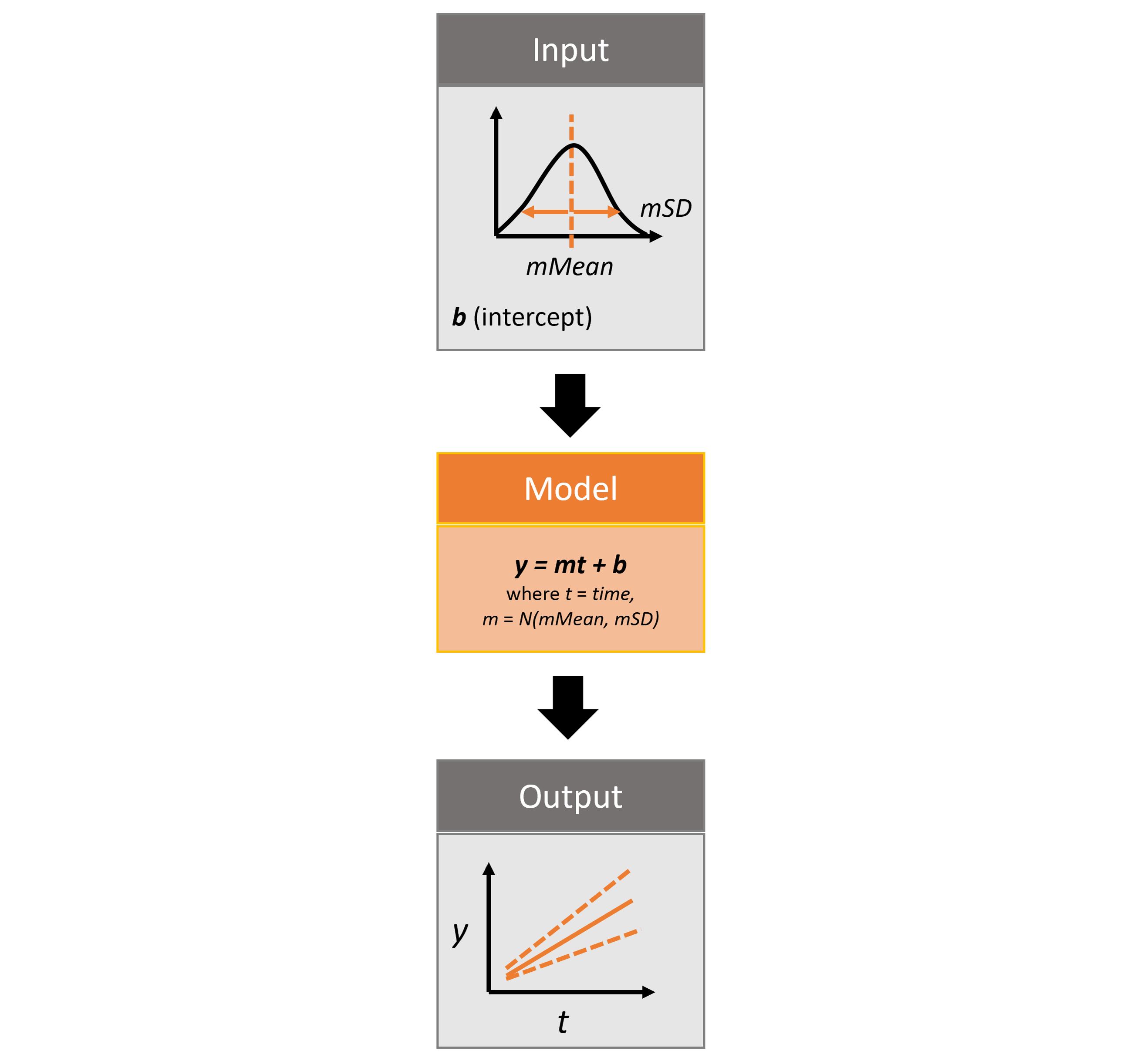
Infographic of helloworldUncertainty package
For more details on the different features of the helloworldUncertainty SyncroSim package, consult the SyncroSim Enhancing a Package: Representing Uncertainty tutorial.
Setup
Install SyncroSim
Before using rsyncrosim you will first need to download and install the SyncroSim software. Versions of SyncroSim exist for both Windows and Linux.
Installing and loading R packages
You will need to install the rsyncrosim R package, either using CRAN or from the rsyncrosim GitHub repository. Versions of rsyncrosim are available for both Windows and Linux.
In a new R script, load the rsyncrosim package.
# Load R package for working with SyncroSim
library(rsyncrosim)
Installing SyncroSim packages using installPackage()
Install helloworldUncertainty using the rynscrosim function installPackage(). This function takes a package name as input and then queries the SyncroSim package server for the specified package.
# Install helloworldUncertainty
installPackage("helloworldUncertainty")
## Package <helloworldUncertainty> installedhelloworldUncertainty should now be included in the package list when we call the package() function:
# Get list of installed packages
package()
## name description version
## 1 helloworldUncertainty Example demonstrating how to use iterations 1.0.0
Connecting R to SyncroSim using session()
Finish setting up the R environment for the rsyncrosim workflow by creating a SyncroSim Session object. Use the session() function to connect R to your installed copy of the SyncroSim software.
mySession <- session("path/to/install_folder")      # Create a Session based SyncroSim install folder
mySession <- session()                              # Using default install folder (Windows only)
mySession                                           # Displays the Session object
## class : Session
## filepath [character]: C:/Program Files/SyncroSim
## silent [logical] : TRUE
## printCmd [logical] : FALSEUse the version() function to ensure you are using the latest version of SyncroSim.
version(mySession)## [1] "2.3.3"Create a modeling workflow
When creating a new modeling workflow from scratch, we need to create objects of the following scopes:
For more information on these scopes, see the Introduction to rsyncrosim vignette.
Set up Library, Project, and Scenario
# Create a new Library
myLibrary <- ssimLibrary(name = "helloworldLibrary.ssim",
                         session = mySession,
                         package = "helloworldUncertainty",
                         overwrite = TRUE)

# Open the default Project
myProject = project(ssimObject = myLibrary, project = "Definitions")

# Create a new Scenario (associated with the default Project)
myScenario = scenario(ssimObject = myProject, scenario = "My first scenario")
View model inputs using datasheet()
View the Datasheets associated with your new Scenario using the datasheet() function from rsyncrosim.
# View all Datasheets associated with a Library, Project, or Scenario
datasheet(myScenario)
## scope name displayName
## 1 scenario helloworldUncertainty_InputDatasheet InputDatasheet
## 2 scenario helloworldUncertainty_OutputDatasheet OutputDatasheet
## 3 scenario helloworldUncertainty_RunControl Run ControlFrom the list of Datasheets above, we can see that there are three Datasheets specific to the helloworldUncertainty package. Let’s view the contents of the input Datasheet as an R data frame.
# View the contents of the input Datasheet for the Scenario
datasheet(myScenario, name = "helloworldUncertainty_InputDatasheet")
## [1] mMean mSD b
## <0 rows> (or 0-length row.names)
Configure model inputs using datasheet() and addRow()
Input Datasheet
Currently our input Scenario Datasheet is empty! We need to add some values to our input Datasheet (InputDatasheet) so we can run our model. First, assign the contents of the input Datasheet to a new data frame variable using datasheet(), then check the columns that need input values.
# Load the input Datasheet to an R data frame
myInputDataframe <- datasheet(myScenario,
                              name = "helloworldUncertainty_InputDatasheet")

# Check the columns of the input data frame
str(myInputDataframe)
## 'data.frame': 0 obs. of 3 variables:
## $ mMean: num
## $ mSD : num
## $ b : numThe input Datasheet requires three values:
-
mMean: the mean of the slope normal distribution. -
mSD: the standard deviation of the slope normal distribution. -
b: the intercept of the linear equation.
Add these values to a new data frame, then use the addRow() function from rsyncrosim to update the input data frame.
# Create input data and add it to the input data frame
myInputRow <- data.frame(mMean = 2, mSD = 4, b = 3)
myInputDataframe <- addRow(myInputDataframe, myInputRow)

# Check values
myInputDataframe
## mMean mSD b
## 1 2 4 3Finally, save the updated R data frame to a SyncroSim Datasheet using saveDatasheet().
# Save input R data frame to a SyncroSim Datasheet
saveDatasheet(ssimObject = myScenario, data = myInputDataframe,
              name = "helloworldUncertainty_InputDatasheet")
## Datasheet <helloworldUncertainty_InputDatasheet> savedRunControl Datasheet
The RunControl Datasheet provides information about how many time steps and iterations to use in the model. Here, we set the number of iterations, as well as the minimum and maximum time steps for our model. The number of iterations we set is equivalent to the number of Monte Carlo realizations, so the greater the number of iterations, the more accurate the range of output values we will obtain. Let’s take a look at the columns that need input values.
# Load RunControl Datasheet to a new R data frame
runSettings <- datasheet(myScenario, name = "helloworldUncertainty_RunControl")

# Check the columns of the RunControl data frame
str(runSettings)
## 'data.frame': 0 obs. of 4 variables:
## $ MinimumIteration: num
## $ MaximumIteration: num
## $ MinimumTimestep : num
## $ MaximumTimestep : numThe RunControl Datasheet requires the following 4 columns:
-
MinimumIteration: starting value of iterations (default=1). -
MaximumIteration: total number of iterations to run the model for. -
MinimumTimestep: the starting time point of the simulation. -
MaximumTimestep: the end time point of the simulation.
We’ll add this information to an R data frame and then add it to the Run Control data frame using addRow(). For this example, we will use only five iterations.
# Create run control data and add it to the run control data frame
runSettingsRow <- data.frame(MinimumIteration = 1,
                             MaximumIteration = 5,
                             MinimumTimestep = 1,
                             MaximumTimestep = 10)
runSettings <- addRow(runSettings, runSettingsRow)

# Check values
runSettings
## MinimumIteration MaximumIteration MinimumTimestep MaximumTimestep
## 1 1 5 1 10Finally, save the R data frame to a SyncroSim Datasheet using saveDatasheet().
# Save RunControl R data frame to a SyncroSim Datasheet
saveDatasheet(ssimObject = myScenario, data = runSettings,
              name = "helloworldUncertainty_RunControl")
## Datasheet <helloworldUncertainty_RunControl> savedRun Scenarios
Setting run parameters with run()
We will now run our Scenario using the run() function in rsyncrosim. If we have a large model and we want to parallelize the run using multiprocessing, we can set the jobs argument to be a value greater than one. Since we are using five iterations in our model, we will set the number of jobs to five so each multiprocessing core will run a single iteration.
# Run the first Scenario we created
myResultScenario <- run(myScenario, jobs = 5)
## [1] "Running scenario [1] My first scenario"Running the original Scenario creates a new Scenario object, known as a Results Scenario, that contains a read-only snapshot of the input Datasheets, as well as the output Datasheets filled with result data. We can view which Scenarios are Results Scenarios using the scenario() function from rsyncrosim.
# Check that we have two Scenarios, and one is a Results Scenario
scenario(myLibrary)
## scenarioId projectId name isResult
## 1 1 1 My first scenario No
## 2 2 1 My first scenario ([1] @ 07-Sep-2021 1:35 PM) Yes
## parentID owner lastModified readOnly mergeDependencies
## 1 NA N/A 2021-09-07 at 1:35 PM No No
## 2 1 N/A 2021-09-07 at 1:35 PM No No
## ignoreDependencies autoGenTags
## 1 NA NA
## 2 NA NAView results
Viewing results with datasheet()
The next step is to view the output Datasheets added to the Result Scenario when it was run. We can load the result tables using the datasheet() function. In this package, the Datasheet containing the results is called “OutputDatasheet”.
# Results of first Scenario
resultsSummary <- datasheet(myResultScenario,
                            name = "helloworldUncertainty_OutputDatasheet")

# View results table
head(resultsSummary)
## Iteration Timestep y
## 1 1 1 4.0171
## 2 1 2 5.0342
## 3 1 3 6.0513
## 4 1 4 7.0684
## 5 1 5 8.0855
## 6 1 6 9.1026Plotting uncertainty in the SyncroSim Windows User Interface
Now that we have run multiple iterations, we can visualize the uncertainty in our results. For this plot, we will plot the average y values over time, while showing the 20th and 80th percentiles.
To create a plot using the Results Scenario we just generated, open the current Library in the User Interface and sync the updates from rsyncrosim using the “refresh” button in the upper toolbar. All the updates made in rsyncrosim should appear in the User Interface. We can now add the Results Scenario to the Results Viewer and create our plot. For more information on generating plots in the User Interface, see the SyncroSim tutorials on creating and customizing charts.
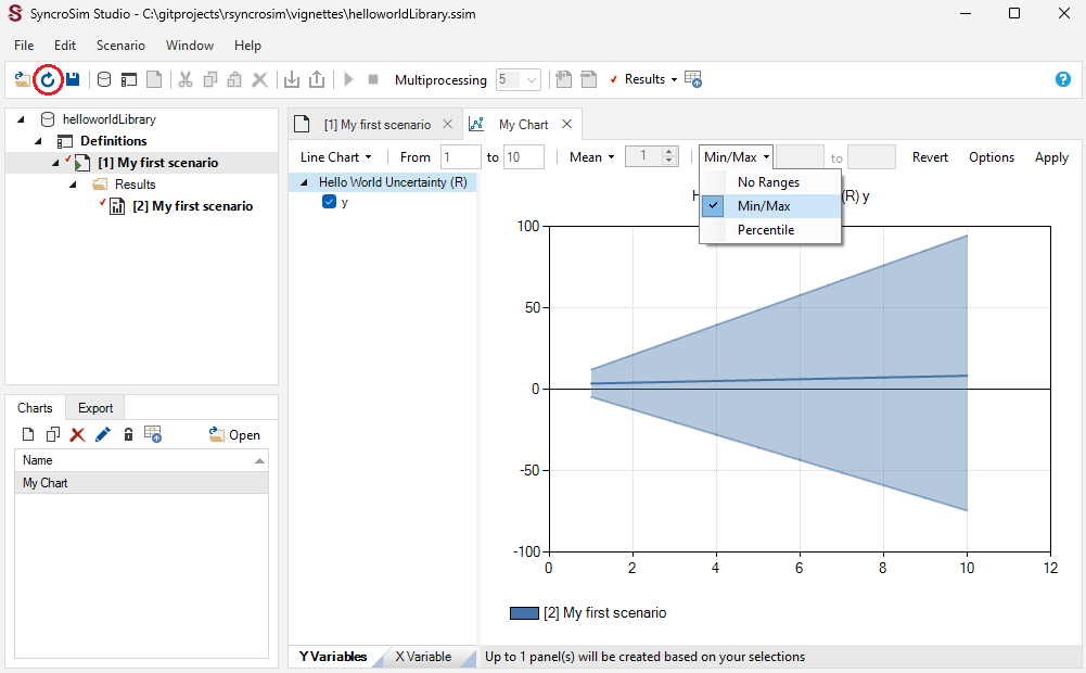
Using rsyncrosim with the SyncroSim Windows User Interface to plot uncertainty