rsyncrosim: introduction to pipelines
Source: vignettes/rsyncrosim_vignette_pipelines.Rmd
rsyncrosim_vignette_pipelines.RmdThis vignette will cover how to use model pipelines using the rsyncrosim package within the SyncroSim software framework. For an overview of SyncroSim and rsyncrosim, as well as a basic usage tutorial for rsyncrosim, see the Introduction to rsyncrosim vignette. To learn how to use iterations in the rsyncrosim interface, see the rsyncrosim: introduction to uncertainty vignette.
SyncroSim Package: helloworldPipeline
To demonstrate how to link models in a pipeline using the rsyncrosim interface, we will need the helloworldPipeline SyncroSim package. helloworldPipeline was designed to be a simple package to introduce pipelines to SyncroSim modeling workflows. Models (i.e. Transformers) connected by pipelines allow the user to implement multiple Transformers in a modeling workflow and access intermediate outputs of a Transformer without having to create multiple Scenarios.
The package takes from the user 3 inputs, mMean, mSD, and b. For each iteration, a value m, representing the slope, is sampled from a normal distribution with mean of mMean and standard deviation of mSD. The b value represents the intercept. In the first model in the pipeline, these input values are run through a linear model, y=mt+b, where t is time, and the y value is returned as output. The second model takes y as input and calculates the cumulative sum of y over time, returning a new variable yCum as output.
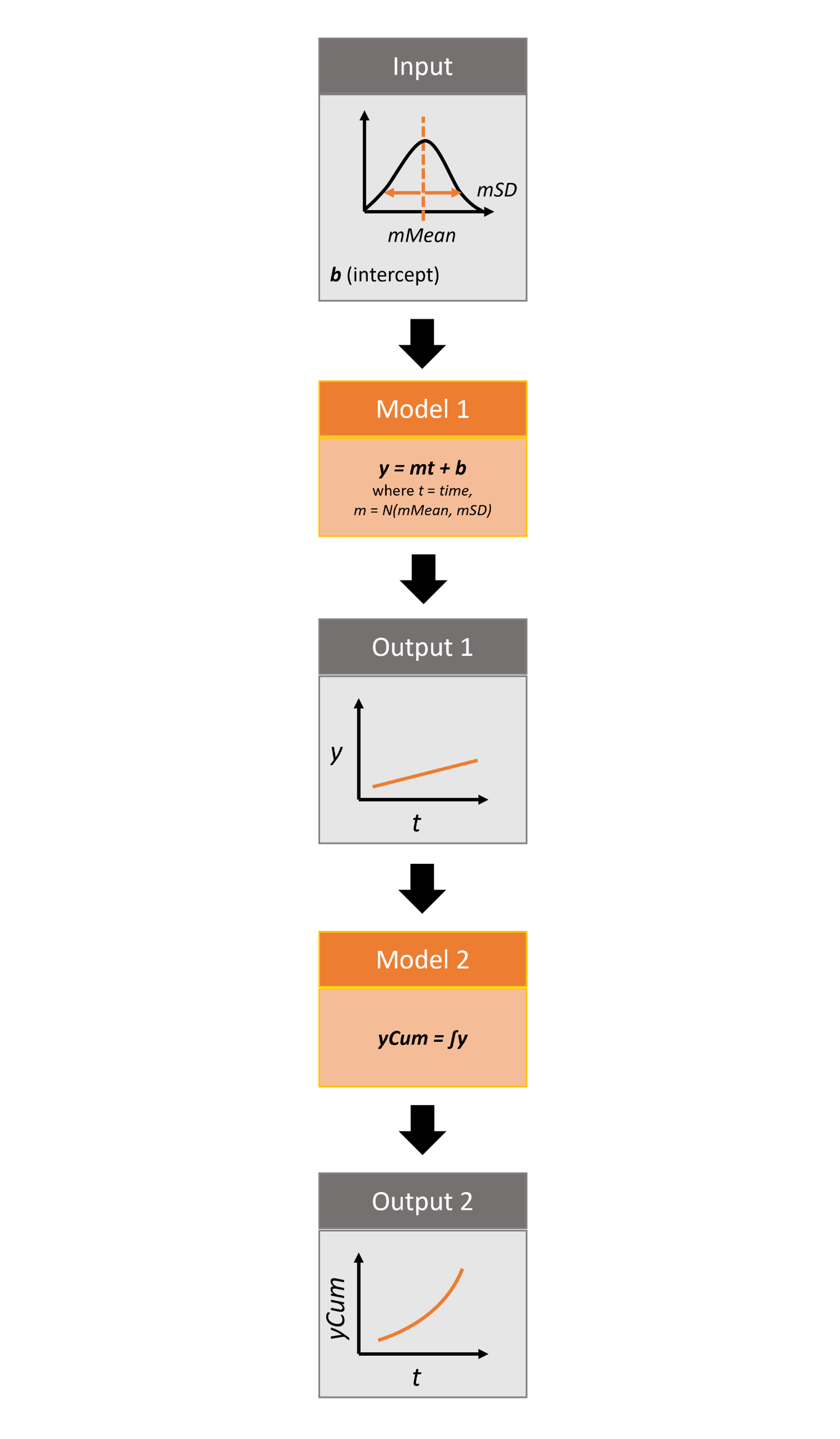
Infographic of helloworldPipeline package
For more details on the different features of the helloworldPipeline SyncroSim package, consult the SyncroSim Enhancing a Package: Linking Models tutorial.
Setup
Install SyncroSim
Before using rsyncrosim you will first need to download and install the SyncroSim software. Versions of SyncroSim exist for both Windows and Linux.
Installing and loading R packages
You will need to install the rsyncrosim R package, either using CRAN or from the rsyncrosim GitHub repository. Versions of rsyncrosim are available for both Windows and Linux.
In a new R script, load the rsyncrosim package.
# Load R package for working with SyncroSim
library(rsyncrosim)
Installing SyncroSim packages using installPackage()
Install helloworldPipeline using the rynscrosim function installPackage(). This function takes a package name as input and then queries the SyncroSim package server for the specified package.
# Install helloworldPipeline
installPackage("helloworldPipeline")
## Package <helloworldPipeline> installedhelloworldPipeline should now be included in the package list returned by the package() function in rsyncrosim:
# Get list of installed packages
package()
## name description version
## 1 helloworldPipeline Example demonstrating how to use pipelines 1.0.0
Connecting R to SyncroSim using session()
Finish setting up the R environment for the rsyncrosim workflow by creating a SyncroSim Session object. Use the session() function to connect R to your installed copy of the SyncroSim software.
mySession <- session("path/to/install_folder")      # Create a Session based SyncroSim install folder
mySession <- session()                              # Using default install folder (Windows only)
mySession                                           # Displays the Session object
## class : Session
## filepath [character]: C:/Program Files/SyncroSim
## silent [logical] : TRUE
## printCmd [logical] : FALSEUse the version() function to ensure you are using the latest version of SyncroSim.
version(mySession)## [1] "2.3.3"Create a modeling workflow
When creating a new modeling workflow from scratch, we need to create objects of the following scopes:
For more information on these scopes, see the Introduction to rsyncrosim vignette.
Set up Library, Project, and Scenario
# Create a new Library
myLibrary <- ssimLibrary(name = "helloworldLibrary.ssim",
                         session = mySession,
                         package = "helloworldPipeline",
                         overwrite = TRUE)

# Open the default Project
myProject = project(ssimObject = myLibrary, project = "Definitions")

# Create a new Scenario (associated with the default Project)
myScenario = scenario(ssimObject = myProject, scenario = "My first scenario")
View model inputs using datasheet()
View the Datasheets associated with your new Scenario using the datasheet() function from rsyncrosim.
# View all Datasheets associated with a Library, Project, or Scenario
datasheet(myScenario)
## scope name displayName
## 1 scenario helloworldPipeline_InputDatasheet InputDatasheet
## 2 scenario helloworldPipeline_IntermediateDatasheet IntermediateDatasheet
## 3 scenario helloworldPipeline_OutputDatasheet OutputDatasheet
## 4 scenario helloworldPipeline_RunControl Run ControlFrom the list of Datasheets above, we can see that there are four Datasheets specific to the helloworldPipeline package, including an Input Datasheet, an Intermediate Datasheet, and an Output Datasheet. These three Datasheets are connected by Transformers. The values from the Input Datasheet are used as the input for the first Transformer, which transforms the input data to output data through a series of model calculations. The output data from the first Transformer is contained within the Intermediate Datasheet. The values from the Intermediate Datasheet are then used as input for the second Transformer. The output from the second Transformer is stored in the Output Datasheet.
Configure model inputs using datasheet() and addRow()
Currently our input Scenario Datasheets are empty! We need to add some values to our input Datasheet (InputDatasheet) and Run Control Datasheet (RunControl) so we can run our model. Since this package also uses pipelines, we also need to add some information to the core Pipeline Datasheet to specify which Transformers are run in which order.
Input Datasheet
First, assign the contents of the input Datasheet to a new data frame variable using datasheet(), then check the columns that need input values.
# Load input Datasheet to a new R data frame
myInputDataframe <- datasheet(myScenario,
                              name = "helloworldPipeline_InputDatasheet")

# Check the columns of the input data frame
str(myInputDataframe)
## 'data.frame': 0 obs. of 3 variables:
## $ mMean: num
## $ mSD : num
## $ b : numThe input Datasheet requires three values:
-
mMean: the mean of the slope normal distribution. -
mSD: the standard deviation of the slope normal distribution. -
b: the intercept of the linear equation.
Add these values to a new data frame, then use the addRow() function from rsyncrosim to update the input data frame
# Create input data and add it to the input data frame
myInputRow <- data.frame(mMean = 2, mSD = 4, b = 3)
myInputDataframe <- addRow(myInputDataframe, myInputRow)

# Check values
myInputDataframe
## mMean mSD b
## 1 2 4 3Finally, save the updated R data frame to a SyncroSim Datasheet using saveDatasheet().
# Save input R data frame to a SyncroSim Datasheet
saveDatasheet(ssimObject = myScenario, data = myInputDataframe,
              name = "helloworldPipeline_InputDatasheet")
## Datasheet <helloworldPipeline_InputDatasheet> savedRunControl Datasheet
The RunControl Datasheet provides information about how many time steps and iterations to use in the model. Here, we set the number of iterations, as well as the minimum and maximum time steps for our model. Let’s take a look at the columns that need input values.
# Load RunControl Datasheet to a new R data frame
runSettings <- datasheet(myScenario, name = "helloworldPipeline_RunControl")

# Check the columns of the RunControl data frame
str(runSettings)
## 'data.frame': 0 obs. of 4 variables:
## $ MinimumIteration: num
## $ MaximumIteration: num
## $ MinimumTimestep : num
## $ MaximumTimestep : numThe RunControl Datasheet requires the following 4 columns:
-
MinimumIteration: starting value of iterations (default=1). -
MaximumIteration: total number of iterations to run the model for. -
MinimumTimestep: the starting time point of the simulation. -
MaximumTimestep: the end time point of the simulation.
We’ll add this information to a new data frame and then add it to the Run Control data frame using addRow().
# Create RunControl data and add it to the RunControl data frame
runSettingsRow <- data.frame(MinimumIteration = 1,
                             MaximumIteration = 5,
                             MinimumTimestep = 1,
                             MaximumTimestep = 10)
runSettings <- addRow(runSettings, runSettingsRow)

# Check values
runSettings
## MinimumIteration MaximumIteration MinimumTimestep MaximumTimestep
## 1 1 5 1 10Finally, save the R data frame to a SyncroSim Datasheet using saveDatasheet().
# Save RunControl R data frame to a SyncroSim Datasheet
saveDatasheet(ssimObject = myScenario, data = runSettings,
              name = "helloworldPipeline_RunControl")
## Datasheet <helloworldPipeline_RunControl> savedPipeline Datasheet
We must modify a third Datasheet to be able to use the output of one Transformer as the input of a second Transformer. To implement pipelines in our package, we need to specify the order in which to run the Transformers in our pipeline by editing the Pipeline Datasheet. The Pipeline Datasheet is part of the built-in SyncroSim core, so we access it using the “core_” prefix with the datasheet() function. From viewing the structure of the Pipeline Datasheet we know that the StageNameID is a factor with two levels: “First Model” and “Second Model”. We will set the data for this Datasheet such that “First Model” is run first, then “Second Model”. This way, the output from “First Model” is used as the input for “Second Model”.
# Load Pipeline Datasheet to a new R data frame
myPipelineDataframe <- datasheet(myScenario, name = "core_Pipeline")

# Check the columns of the Pipeline data frame
str(myPipelineDataframe)

# Create Pipeline data and add it to the Pipeline data frame
myPipelineRow <- data.frame(StageNameID = c("First Model", "Second Model"),
                            RunOrder = c(1, 2))

myPipelineDataframe <- addRow(myPipelineDataframe, myPipelineRow)

# Check values
myPipelineDataframe

# Save Pipeline R data frame to a SyncroSim Datasheet
saveDatasheet(ssimObject = myScenario, data = myPipelineDataframe,
              name = "core_Pipeline")
Run Scenarios
Setting run parameters with run()
We will now run our Scenario using the run() function in rsyncrosim. If we have a large modeling workflow and we want to parallelize the run using multiprocessing, we can set the jobs argument to be a value greater than one.
# Run the first Scenario we created
myResultScenario <- run(myScenario, jobs = 5)
## [1] "Running scenario [1] My first scenario"Once the run is complete, we can compare the original Scenario to the Results Scenario to see which Datasheets have been modified. Using the datasheet() function with the optional argument set to TRUE, we see that data has been added to both the Intermediate and Output Datasheets after running the Scenario (see data column below).
# Datasheets for original Scenario
datasheet(myScenario, optional = TRUE)
## scope package name
## 1 scenario helloworldPipeline helloworldPipeline_InputDatasheet
## 2 scenario helloworldPipeline helloworldPipeline_IntermediateDatasheet
## 3 scenario helloworldPipeline helloworldPipeline_OutputDatasheet
## 4 scenario helloworldPipeline helloworldPipeline_RunControl
## displayName isSingle isOutput data scenario
## 1 InputDatasheet TRUE FALSE TRUE 1
## 2 IntermediateDatasheet FALSE FALSE FALSE 1
## 3 OutputDatasheet FALSE FALSE FALSE 1
## 4 Run Control TRUE FALSE TRUE 1
# Datasheets for Results Scenario
datasheet(myResultScenario, optional = TRUE)
## scope package name
## 1 scenario helloworldPipeline helloworldPipeline_InputDatasheet
## 2 scenario helloworldPipeline helloworldPipeline_IntermediateDatasheet
## 3 scenario helloworldPipeline helloworldPipeline_OutputDatasheet
## 4 scenario helloworldPipeline helloworldPipeline_RunControl
## displayName isSingle isOutput data scenario
## 1 InputDatasheet TRUE FALSE TRUE 1
## 2 IntermediateDatasheet FALSE FALSE TRUE 1
## 3 OutputDatasheet FALSE FALSE FALSE 1
## 4 Run Control TRUE FALSE TRUE 1View results
The next step is to view the output Datasheets added to the Result Scenario when it was run.
Viewing intermediate results with datasheet()
First, we will view the intermediate output Datasheet from the Results Scenario. We can load the result tables using the datasheet() function. The Intermediate Datasheet corresponds to the results from the first model.
# Results of first Scenario
resultsSummary <- datasheet(myResultScenario,
                            name = "helloworldPipeline_IntermediateDatasheet")

# View results table
head(resultsSummary)
## Iteration Timestep y
## 1 1 1 8.4741
## 2 1 2 13.9481
## 3 1 3 19.4222
## 4 1 4 24.8963
## 5 1 5 30.3704
## 6 1 6 35.8444We can see that for every timestep in an iteration we have a new value of y corresponding to y=mt+b.
Viewing final results with datasheet()
Now, we will view the final output Datasheet from the Results Scenario. Again, we will use datasheet() to load the result table. The Output Datasheet corresponds to the results from the second model.
# Results of first Scenario
resultsSummary <- datasheet(myResultScenario,
                            name = "helloworldPipeline_OutputDatasheet")

# View results table
head(resultsSummary)
## [1] Iteration Timestep yCum
## <0 rows> (or 0-length row.names)We can see for each timestep in an iteration, we have a new value of yCum, representing the cumulative value of y over time.